Models and Fitting (astropy.modeling)

Introduction

astropy.modeling provides a framework for representing models and performing model evaluation and fitting. It currently supports 1-D and 2-D models and fitting with parameter constraints.

It is designed to be easily extensible and flexible. Models do not reference fitting algorithms explicitly and new fitting algorithms may be added without changing the existing models (though not all models can be used with all fitting algorithms due to constraints such as model linearity).

The goal is to eventually provide a rich toolset of models and fitters such that most users will not need to define new model classes, nor special purpose fitting routines (while making it reasonably easy to do when necessary).

Note

astropy.modeling is currently a work-in-progress, and thus it is likely there will still be API changes in later versions of Astropy. Backwards compatibility support between versions will still be maintained as much as possible, but new features and enhancements are coming in future versions. If you have specific ideas for how it might be improved, feel free to let us know on the astropy-dev mailing list or at http://feedback.astropy.org

Getting started

The examples here use the predefined models and assume the following modules have been imported:

>>> import numpy as np
>>> from astropy.modeling import models, fitting

Using Models

The astropy.modeling package defines a number of models that are collected under a single namespace as astropy.modeling.models. Models behave like parametrized functions:

>>> from astropy.modeling import models
>>> g = models.Gaussian1D(amplitude=1.2, mean=0.9, stddev=0.5)
>>> print(g)
Model: Gaussian1D
Inputs: ('x',)
Outputs: ('y',)
Model set size: 1
Parameters:
    amplitude mean stddev
    --------- ---- ------
          1.2  0.9    0.5

Model parameters can be accessed as attributes:

>>> g.amplitude
Parameter('amplitude', value=1.2)
>>> g.mean
Parameter('mean', value=0.9)
>>> g.stddev  
Parameter('stddev', value=0.5, bounds=(1.1754943508222875e-38, None))

and can also be updated via those attributes:

>>> g.amplitude = 0.8
>>> g.amplitude
Parameter('amplitude', value=0.8)

Models can be evaluated by calling them as functions:

>>> g(0.1)
0.22242984036255528
>>> g(np.linspace(0.5, 1.5, 7))  
array([0.58091923, 0.71746405, 0.7929204 , 0.78415894, 0.69394278,
       0.54952605, 0.3894018 ])

As the above example demonstrates, in general most models evaluate array-like inputs according to the standard Numpy broadcasting rules for arrays.

Models can therefore already be useful to evaluate common functions, independently of the fitting features of the package.

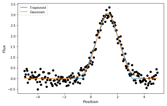
Simple 1-D model fitting

In this section, we look at a simple example of fitting a Gaussian to a simulated dataset. We use the Gaussian1D and Trapezoid1D models and the LevMarLSQFitter fitter to fit the data:

import numpy as np
import matplotlib.pyplot as plt
from astropy.modeling import models, fitting

# Generate fake data
np.random.seed(0)
x = np.linspace(-5., 5., 200)
y = 3 * np.exp(-0.5 * (x - 1.3)**2 / 0.8**2)
y += np.random.normal(0., 0.2, x.shape)

# Fit the data using a box model.
# Bounds are not really needed but included here to demonstrate usage.
t_init = models.Trapezoid1D(amplitude=1., x_0=0., width=1., slope=0.5,
                            bounds={"x_0": (-5., 5.)})
fit_t = fitting.LevMarLSQFitter()
t = fit_t(t_init, x, y)

# Fit the data using a Gaussian
g_init = models.Gaussian1D(amplitude=1., mean=0, stddev=1.)
fit_g = fitting.LevMarLSQFitter()
g = fit_g(g_init, x, y)

# Plot the data with the best-fit model
plt.figure(figsize=(8,5))
plt.plot(x, y, 'ko')
plt.plot(x, t(x), label='Trapezoid')
plt.plot(x, g(x), label='Gaussian')
plt.xlabel('Position')
plt.ylabel('Flux')
plt.legend(loc=2)

(png, svg, pdf)

As shown above, once instantiated, the fitter class can be used as a function that takes the initial model (t_init or g_init) and the data values (x and y), and returns a fitted model (t or g).

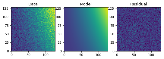
Simple 2-D model fitting

Similarly to the 1-D example, we can create a simulated 2-D data dataset, and fit a polynomial model to it. This could be used for example to fit the background in an image.

import warnings
import numpy as np
import matplotlib.pyplot as plt
from astropy.modeling import models, fitting

# Generate fake data
np.random.seed(0)
y, x = np.mgrid[:128, :128]
z = 2. * x ** 2 - 0.5 * x ** 2 + 1.5 * x * y - 1.
z += np.random.normal(0., 0.1, z.shape) * 50000.

# Fit the data using astropy.modeling
p_init = models.Polynomial2D(degree=2)
fit_p = fitting.LevMarLSQFitter()

with warnings.catch_warnings():
    # Ignore model linearity warning from the fitter
    warnings.simplefilter('ignore')
    p = fit_p(p_init, x, y, z)

# Plot the data with the best-fit model
plt.figure(figsize=(8, 2.5))
plt.subplot(1, 3, 1)
plt.imshow(z, origin='lower', interpolation='nearest', vmin=-1e4, vmax=5e4)
plt.title("Data")
plt.subplot(1, 3, 2)
plt.imshow(p(x, y), origin='lower', interpolation='nearest', vmin=-1e4,
           vmax=5e4)
plt.title("Model")
plt.subplot(1, 3, 3)
plt.imshow(z - p(x, y), origin='lower', interpolation='nearest', vmin=-1e4,
           vmax=5e4)
plt.title("Residual")

(png, svg, pdf)

A list of models is provided in the Reference/API section. The fitting framework includes many useful features that are not demonstrated here, such as weighting of datapoints, fixing or linking parameters, and placing lower or upper limits on parameters. For more information on these, take a look at the Fitting Models to Data documentation.

Model sets

In some cases it is necessary to describe many models of the same type but with different sets of parameter values. This could be done simply by instantiating as many instances of a Model as are needed. But that can be inefficient for a large number of models. To that end, all model classes in astropy.modeling can also be used to represent a model set which is a collection of models of the same type, but with different values for their parameters.

To instantiate a model set, use argument n_models=N where N is the number of models in the set when constructing the model. The value of each parameter must be a list or array of length N, such that each item in the array corresponds to one model in the set:

>>> g = models.Gaussian1D(amplitude=[1, 2], mean=[0, 0],
...                       stddev=[0.1, 0.2], n_models=2)
>>> print(g)
Model: Gaussian1D
Inputs: ('x',)
Outputs: ('y',)
Model set size: 2
Parameters:
    amplitude mean stddev
    --------- ---- ------
          1.0  0.0    0.1
          2.0  0.0    0.2

This is equivalent to two Gaussians with the parameters amplitude=1, mean=0, stddev=0.1 and amplitude=2, mean=0, stddev=0.2 respectively. When printing the model the parameter values are displayed as a table, with each row corresponding to a single model in the set.

The number of models in a model set can be determined using the len builtin:

>>> len(g)
2

Single models have a length of 1, and are not considered a model set as such.

When evaluating a model set, by default the input must be the same length as the number of models, with one input per model:

>>> g([0, 0.1])  
array([1.        , 1.76499381])

The result is an array with one result per model in the set. It is also possible to broadcast a single value to all models in the set:

>>> g(0)  
array([1., 2.])

Model sets are used primarily for fitting, allowing a large number of models of the same type to be fitted simultaneously (and independently from each other) to some large set of inputs. For example, fitting a polynomial to the time response of each pixel in a data cube. This can greatly speed up the fitting process, especially for linear models.

Compound models

New in version 1.0: This feature is experimental and expected to see significant further development, but the basic usage is stable and expected to see wide use.

While the Astropy modeling package makes it very easy to define new models either from existing functions, or by writing a Model subclass, an additional way to create new models is by combining them using arithmetic expressions. This works with models built into Astropy, and most user-defined models as well. For example, it is possible to create a superposition of two Gaussians like so:

>>> from astropy.modeling import models
>>> g1 = models.Gaussian1D(1, 0, 0.2)
>>> g2 = models.Gaussian1D(2.5, 0.5, 0.1)
>>> g1_plus_2 = g1 + g2

The resulting object g1_plus_2 is itself a new model. Evaluating, say, g1_plus_2(0.25) is the same as evaluating g1(0.25) + g2(0.25):

>>> g1_plus_2(0.25)  
0.5676756958301329
>>> g1_plus_2(0.25) == g1(0.25) + g2(0.25)
True

This model can be further combined with other models in new expressions.

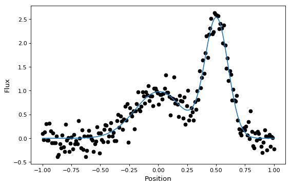
These new compound models can also be fitted to data, like most other models (though this currently requires one of the non-linear fitters):

import numpy as np
import matplotlib.pyplot as plt
from astropy.modeling import models, fitting

# Generate fake data
np.random.seed(42)
g1 = models.Gaussian1D(1, 0, 0.2)
g2 = models.Gaussian1D(2.5, 0.5, 0.1)
x = np.linspace(-1, 1, 200)
y = g1(x) + g2(x) + np.random.normal(0., 0.2, x.shape)

# Now to fit the data create a new superposition with initial
# guesses for the parameters:
gg_init = models.Gaussian1D(1, 0, 0.1) + models.Gaussian1D(2, 0.5, 0.1)
fitter = fitting.SLSQPLSQFitter()
gg_fit = fitter(gg_init, x, y)

# Plot the data with the best-fit model
plt.figure(figsize=(8,5))
plt.plot(x, y, 'ko')
plt.plot(x, gg_fit(x))
plt.xlabel('Position')
plt.ylabel('Flux')

(png, svg, pdf)

This works for 1-D models, 2-D models, and combinations thereof, though there are some complexities involved in correctly matching up the inputs and outputs of all models used to build a compound model. You can learn more details in the Compound Models documentation.

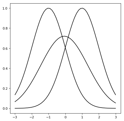
Astropy models also support convolution through the function convolve_models, which returns a compound model.

For instance, the convolution of two Gaussian functions is also a Gaussian function in which the resulting mean (variance) is the sum of the means (variances) of each Gaussian.

import numpy as np
import matplotlib.pyplot as plt
from astropy.modeling import models
from astropy.convolution import convolve_models

g1 = models.Gaussian1D(1, -1, 1)
g2 = models.Gaussian1D(1, 1, 1)
g3 = convolve_models(g1, g2)

x = np.linspace(-3, 3, 50)
plt.plot(x, g1(x), 'k-')
plt.plot(x, g2(x), 'k-')
plt.plot(x, g3(x), 'k-')

(png, svg, pdf)

Fitting masked data

New in version 2.0.4.

When astropy.modeling.fitting.LinearLSQFitter is provided with the dependent co-ordinate values as a numpy.ma.MaskedArray, it ignores any masked values when performing the fit:

>>> p_init = models.Polynomial1D(degree=1)
>>> x = np.arange(10)
>>> y = np.ma.masked_array(2*x+1, mask=np.zeros_like(x))
>>> y[7] = 100.       # simulate spurious value
>>> y.mask[7] = True
>>> fitter = fitting.LinearLSQFitter()
>>> p = fitter(p_init, x, y)
>>> print('Fit intercept={:.3f}, slope={:.3f}'.format(p.c0.value, p.c1.value))  
Fit intercept=1.000, slope=2.000

At present, the non-linear fitters do not distinguish between good and bad values in this way.

Note that model set fitting is currently about an order of magnitude slower in the presence of masked values, because the matrix equation has to be solved for each model separately, on their respective co-ordinate grids. This is still an order of magnitude faster than fitting separate model instances, however. Supplying a numpy.ma.MaskedArray without any bad (True) mask values produces the normal, faster behavior.

Using astropy.modeling

• Instantiating and Evaluating Models
• Parameters
• Fitting Models to Data
• Compound Models
• Defining New Model Classes
• Defining New Fitter Classes
• Using a Custom Statistic Function
• Efficient Model Rendering with Bounding Boxes
• Algorithms
• Support for units and quantities

Performance Tips

Initializing a compound model with many constituent models can be time consuming. If your code uses the same compound model repeatedly consider initializing it once and reusing the model.

Consider the performance tips that apply to quantities when initializing and evaluating models with quantities.

Reference/API

astropy.modeling Package

This subpackage provides a framework for representing models and performing model evaluation and fitting. It supports 1D and 2D models and fitting with parameter constraints. It has some predefined models and fitting routines.

Functions

custom_model(\*args[, fit_deriv])	Create a model from a user defined function.
is_separable(transform)	A separability test for the outputs of a transform.
separability_matrix(transform)	Compute the correlation between outputs and inputs.

Classes

Fittable1DModel(*args[, meta, name])	Base class for one-dimensional fittable models.
Fittable2DModel(*args[, meta, name])	Base class for two-dimensional fittable models.
FittableModel(*args[, meta, name])	Base class for models that can be fitted using the built-in fitting algorithms.
InputParameterError	Used for incorrect input parameter values and definitions.
Model(*args[, meta, name])	Base class for all models.
ModelDefinitionError	Used for incorrect models definitions
Parameter([name, description, default, …])	Wraps individual parameters.
ParameterError	Generic exception class for all exceptions pertaining to Parameters.

Class Inheritance Diagram

astropy.modeling.functional_models Module

Mathematical models.

Classes

AiryDisk2D([amplitude, x_0, y_0, radius])	Two dimensional Airy disk model.
Moffat1D([amplitude, x_0, gamma, alpha])	One dimensional Moffat model.
Moffat2D([amplitude, x_0, y_0, gamma, alpha])	Two dimensional Moffat model.
Box1D([amplitude, x_0, width])	One dimensional Box model.
Box2D([amplitude, x_0, y_0, x_width, y_width])	Two dimensional Box model.
Const1D([amplitude])	One dimensional Constant model.
Const2D([amplitude])	Two dimensional Constant model.
Ellipse2D([amplitude, x_0, y_0, a, b, theta])	A 2D Ellipse model.
Disk2D([amplitude, x_0, y_0, R_0])	Two dimensional radial symmetric Disk model.
Gaussian1D([amplitude, mean, stddev])	One dimensional Gaussian model.
Gaussian2D([amplitude, x_mean, y_mean, …])	Two dimensional Gaussian model.
Linear1D([slope, intercept])	One dimensional Line model.
Lorentz1D([amplitude, x_0, fwhm])	One dimensional Lorentzian model.
MexicanHat1D([amplitude, x_0, sigma])	One dimensional Mexican Hat model.
MexicanHat2D([amplitude, x_0, y_0, sigma])	Two dimensional symmetric Mexican Hat model.
RedshiftScaleFactor([z])	One dimensional redshift scale factor model.
Multiply([factor])	Multiply a model by a quantity or number.
Planar2D([slope_x, slope_y, intercept])	Two dimensional Plane model.
Scale([factor])	Multiply a model by a dimensionless factor.
Sersic1D([amplitude, r_eff, n])	One dimensional Sersic surface brightness profile.
Sersic2D([amplitude, r_eff, n, x_0, y_0, …])	Two dimensional Sersic surface brightness profile.
Shift([offset])	Shift a coordinate.
Sine1D([amplitude, frequency, phase])	One dimensional Sine model.
Trapezoid1D([amplitude, x_0, width, slope])	One dimensional Trapezoid model.
TrapezoidDisk2D([amplitude, x_0, y_0, R_0, …])	Two dimensional circular Trapezoid model.
Ring2D([amplitude, x_0, y_0, r_in, width, r_out])	Two dimensional radial symmetric Ring model.
Voigt1D([x_0, amplitude_L, fwhm_L, fwhm_G])	One dimensional model for the Voigt profile.

Class Inheritance Diagram

astropy.modeling.powerlaws Module

Power law model variants

Classes

PowerLaw1D([amplitude, x_0, alpha])	One dimensional power law model.
BrokenPowerLaw1D([amplitude, x_break, …])	One dimensional power law model with a break.
SmoothlyBrokenPowerLaw1D([amplitude, …])	One dimensional smoothly broken power law model.
ExponentialCutoffPowerLaw1D([amplitude, …])	One dimensional power law model with an exponential cutoff.
LogParabola1D([amplitude, x_0, alpha, beta])	One dimensional log parabola model (sometimes called curved power law).

Class Inheritance Diagram

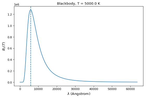
astropy.modeling.blackbody Module

Model and functions related to blackbody radiation.

Blackbody Radiation

Blackbody flux is calculated with Planck law (Rybicki & Lightman 1979):

\[ \begin{align}\begin{aligned}B_{\lambda}(T) = \frac{2 h c^{2} / \lambda^{5}}{exp(h c / \lambda k T) - 1}\\B_{\nu}(T) = \frac{2 h \nu^{3} / c^{2}}{exp(h \nu / k T) - 1}\end{aligned}\end{align} \]

where the unit of \(B_{\lambda}(T)\) is \(erg \; s^{-1} cm^{-2} \mathring{A}^{-1} sr^{-1}\), and \(B_{\nu}(T)\) is \(erg \; s^{-1} cm^{-2} Hz^{-1} sr^{-1}\). blackbody_lambda() and blackbody_nu() calculate the blackbody flux for \(B_{\lambda}(T)\) and \(B_{\nu}(T)\), respectively.

For blackbody representation as a model, see BlackBody1D.

Examples

>>> import numpy as np
>>> from astropy import units as u
>>> from astropy.modeling.blackbody import blackbody_lambda, blackbody_nu

Calculate blackbody flux for 5000 K at 100 and 10000 Angstrom while suppressing any Numpy warnings:

>>> wavelengths = [100, 10000] * u.AA
>>> temperature = 5000 * u.K
>>> with np.errstate(all='ignore'):
...     flux_lam = blackbody_lambda(wavelengths, temperature)
...     flux_nu = blackbody_nu(wavelengths, temperature)
>>> flux_lam  
<Quantity [  1.27452545e-108,  7.10190526e+005] erg / (Angstrom cm2 s sr)>
>>> flux_nu  
<Quantity [  4.25135927e-123,  2.36894060e-005] erg / (cm2 Hz s sr)>

Alternatively, the same results for flux_nu can be computed using BlackBody1D with blackbody representation as a model. The difference between this and the former approach is in one additional step outlined as follows:

>>> from astropy import constants as const
>>> from astropy.modeling import models
>>> temperature = 5000 * u.K
>>> bolometric_flux = const.sigma_sb * temperature ** 4 / np.pi
>>> bolometric_flux.to(u.erg / (u.cm * u.cm * u.s))  
<Quantity 1.12808367e+10 erg / (cm2 s)>
>>> wavelengths = [100, 10000] * u.AA
>>> bb_astro = models.BlackBody1D(temperature, bolometric_flux=bolometric_flux)
>>> bb_astro(wavelengths).to(u.erg / (u.cm * u.cm * u.Hz * u.s)) / u.sr  
<Quantity [4.25102471e-123, 2.36893879e-005] erg / (cm2 Hz s sr)>

where bb_astro(wavelengths) computes the equivalent result as flux_nu above.

Plot a blackbody spectrum for 5000 K:

(png, svg, pdf)

Note that an array of temperatures can also be given instead of a single temperature. In this case, the Numpy broadcasting rules apply: for instance, if the frequency and temperature have the same shape, the output will have this shape too, while if the frequency is a 2-d array with shape (n, m) and the temperature is an array with shape (m,), the output will have a shape (n, m).

See Also

Rybicki, G. B., & Lightman, A. P. 1979, Radiative Processes in Astrophysics (New York, NY: Wiley)

Functions

blackbody_nu(in_x, temperature)	Calculate blackbody flux per steradian, \(B_{\nu}(T)\).
blackbody_lambda(in_x, temperature)	Like blackbody_nu() but for \(B_{\lambda}(T)\).

Classes

BlackBody1D([temperature, bolometric_flux])

One dimensional blackbody model.

Class Inheritance Diagram

astropy.modeling.polynomial Module

This module contains models representing polynomials and polynomial series.

Classes

Chebyshev1D(degree[, domain, window, …])	Univariate Chebyshev series.
Chebyshev2D(x_degree, y_degree[, x_domain, …])	Bivariate Chebyshev series..
Hermite1D(degree[, domain, window, …])	Univariate Hermite series.
Hermite2D(x_degree, y_degree[, x_domain, …])	Bivariate Hermite series.
InverseSIP(ap_order, bp_order[, ap_coeff, …])	Inverse Simple Imaging Polynomial
Legendre1D(degree[, domain, window, …])	Univariate Legendre series.
Legendre2D(x_degree, y_degree[, x_domain, …])	Bivariate Legendre series.
Polynomial1D(degree[, domain, window, …])	1D Polynomial model.
Polynomial2D(degree[, x_domain, y_domain, …])	2D Polynomial model.
SIP(crpix, a_order, b_order[, a_coeff, …])	Simple Imaging Polynomial (SIP) model.
OrthoPolynomialBase(x_degree, y_degree[, …])	This is a base class for the 2D Chebyshev and Legendre models.
PolynomialModel(degree[, n_models, …])	Base class for polynomial models.

Class Inheritance Diagram

astropy.modeling.projections Module

Implements projections–particularly sky projections defined in WCS Paper II [1].

All angles are set and and displayed in degrees but internally computations are performed in radians. All functions expect inputs and outputs degrees.

References

1

Calabretta, M.R., Greisen, E.W., 2002, A&A, 395, 1077 (Paper II)

Classes

Projection(*args[, meta, name])	Base class for all sky projections.
Pix2SkyProjection(*args[, meta, name])	Base class for all Pix2Sky projections.
Sky2PixProjection(*args[, meta, name])	Base class for all Sky2Pix projections.
Zenithal(*args[, meta, name])	Base class for all Zenithal projections.
Cylindrical(*args[, meta, name])	Base class for Cylindrical projections.
PseudoCylindrical(*args[, meta, name])	Base class for pseudocylindrical projections.
Conic(*args[, meta, name])	Base class for conic projections.
PseudoConic(*args[, meta, name])	Base class for pseudoconic projections.
QuadCube(*args[, meta, name])	Base class for quad cube projections.
HEALPix(*args[, meta, name])	Base class for HEALPix projections.
AffineTransformation2D([matrix, translation])	Perform an affine transformation in 2 dimensions.
Pix2Sky_ZenithalPerspective([mu, gamma])	Zenithal perspective projection - pixel to sky.
Sky2Pix_ZenithalPerspective([mu, gamma])	Zenithal perspective projection - sky to pixel.
Pix2Sky_SlantZenithalPerspective([mu, phi0, …])	Slant zenithal perspective projection - pixel to sky.
Sky2Pix_SlantZenithalPerspective([mu, phi0, …])	Zenithal perspective projection - sky to pixel.
Pix2Sky_Gnomonic(*args[, meta, name])	Gnomonic projection - pixel to sky.
Sky2Pix_Gnomonic(*args[, meta, name])	Gnomonic Projection - sky to pixel.
Pix2Sky_Stereographic(*args[, meta, name])	Stereographic Projection - pixel to sky.
Sky2Pix_Stereographic(*args[, meta, name])	Stereographic Projection - sky to pixel.
Pix2Sky_SlantOrthographic([xi, eta])	Slant orthographic projection - pixel to sky.
Sky2Pix_SlantOrthographic([xi, eta])	Slant orthographic projection - sky to pixel.
Pix2Sky_ZenithalEquidistant(*args[, meta, name])	Zenithal equidistant projection - pixel to sky.
Sky2Pix_ZenithalEquidistant(*args[, meta, name])	Zenithal equidistant projection - sky to pixel.
Pix2Sky_ZenithalEqualArea(*args[, meta, name])	Zenithal equidistant projection - pixel to sky.
Sky2Pix_ZenithalEqualArea(*args[, meta, name])	Zenithal equidistant projection - sky to pixel.
Pix2Sky_Airy([theta_b])	Airy projection - pixel to sky.
Sky2Pix_Airy([theta_b])	Airy - sky to pixel.
Pix2Sky_CylindricalPerspective([mu, lam])	Cylindrical perspective - pixel to sky.
Sky2Pix_CylindricalPerspective([mu, lam])	Cylindrical Perspective - sky to pixel.
Pix2Sky_CylindricalEqualArea([lam])	Cylindrical equal area projection - pixel to sky.
Sky2Pix_CylindricalEqualArea([lam])	Cylindrical equal area projection - sky to pixel.
Pix2Sky_PlateCarree(*args[, meta, name])	Plate carrée projection - pixel to sky.
Sky2Pix_PlateCarree(*args[, meta, name])	Plate carrée projection - sky to pixel.
Pix2Sky_Mercator(*args[, meta, name])	Mercator - pixel to sky.
Sky2Pix_Mercator(*args[, meta, name])	Mercator - sky to pixel.
Pix2Sky_SansonFlamsteed(*args[, meta, name])	Sanson-Flamsteed projection - pixel to sky.
Sky2Pix_SansonFlamsteed(*args[, meta, name])	Sanson-Flamsteed projection - sky to pixel.
Pix2Sky_Parabolic(*args[, meta, name])	Parabolic projection - pixel to sky.
Sky2Pix_Parabolic(*args[, meta, name])	Parabolic projection - sky to pixel.
Pix2Sky_Molleweide(*args[, meta, name])	Molleweide’s projection - pixel to sky.
Sky2Pix_Molleweide(*args[, meta, name])	Molleweide’s projection - sky to pixel.
Pix2Sky_HammerAitoff(*args[, meta, name])	Hammer-Aitoff projection - pixel to sky.
Sky2Pix_HammerAitoff(*args[, meta, name])	Hammer-Aitoff projection - sky to pixel.
Pix2Sky_ConicPerspective([sigma, delta])	Colles’ conic perspective projection - pixel to sky.
Sky2Pix_ConicPerspective([sigma, delta])	Colles’ conic perspective projection - sky to pixel.
Pix2Sky_ConicEqualArea([sigma, delta])	Alber’s conic equal area projection - pixel to sky.
Sky2Pix_ConicEqualArea([sigma, delta])	Alber’s conic equal area projection - sky to pixel.
Pix2Sky_ConicEquidistant([sigma, delta])	Conic equidistant projection - pixel to sky.
Sky2Pix_ConicEquidistant([sigma, delta])	Conic equidistant projection - sky to pixel.
Pix2Sky_ConicOrthomorphic([sigma, delta])	Conic orthomorphic projection - pixel to sky.
Sky2Pix_ConicOrthomorphic([sigma, delta])	Conic orthomorphic projection - sky to pixel.
Pix2Sky_BonneEqualArea([theta1])	Bonne’s equal area pseudoconic projection - pixel to sky.
Sky2Pix_BonneEqualArea([theta1])	Bonne’s equal area pseudoconic projection - sky to pixel.
Pix2Sky_Polyconic(*args[, meta, name])	Polyconic projection - pixel to sky.
Sky2Pix_Polyconic(*args[, meta, name])	Polyconic projection - sky to pixel.
Pix2Sky_TangentialSphericalCube(*args[, …])	Tangential spherical cube projection - pixel to sky.
Sky2Pix_TangentialSphericalCube(*args[, …])	Tangential spherical cube projection - sky to pixel.
Pix2Sky_COBEQuadSphericalCube(*args[, meta, …])	COBE quadrilateralized spherical cube projection - pixel to sky.
Sky2Pix_COBEQuadSphericalCube(*args[, meta, …])	COBE quadrilateralized spherical cube projection - sky to pixel.
Pix2Sky_QuadSphericalCube(*args[, meta, name])	Quadrilateralized spherical cube projection - pixel to sky.
Sky2Pix_QuadSphericalCube(*args[, meta, name])	Quadrilateralized spherical cube projection - sky to pixel.
Pix2Sky_HEALPix([H, X])	HEALPix - pixel to sky.
Sky2Pix_HEALPix([H, X])	HEALPix projection - sky to pixel.
Pix2Sky_HEALPixPolar(*args[, meta, name])	HEALPix polar, aka “butterfly” projection - pixel to sky.
Sky2Pix_HEALPixPolar(*args[, meta, name])	HEALPix polar, aka “butterfly” projection - pixel to sky.
Pix2Sky_AZP	alias of astropy.modeling.projections.Pix2Sky_ZenithalPerspective
Sky2Pix_AZP	alias of astropy.modeling.projections.Sky2Pix_ZenithalPerspective
Pix2Sky_SZP	alias of astropy.modeling.projections.Pix2Sky_SlantZenithalPerspective
Sky2Pix_SZP	alias of astropy.modeling.projections.Sky2Pix_SlantZenithalPerspective
Pix2Sky_TAN	alias of astropy.modeling.projections.Pix2Sky_Gnomonic
Sky2Pix_TAN	alias of astropy.modeling.projections.Sky2Pix_Gnomonic
Pix2Sky_STG	alias of astropy.modeling.projections.Pix2Sky_Stereographic
Sky2Pix_STG	alias of astropy.modeling.projections.Sky2Pix_Stereographic
Pix2Sky_SIN	alias of astropy.modeling.projections.Pix2Sky_SlantOrthographic
Sky2Pix_SIN	alias of astropy.modeling.projections.Sky2Pix_SlantOrthographic
Pix2Sky_ARC	alias of astropy.modeling.projections.Pix2Sky_ZenithalEquidistant
Sky2Pix_ARC	alias of astropy.modeling.projections.Sky2Pix_ZenithalEquidistant
Pix2Sky_ZEA	alias of astropy.modeling.projections.Pix2Sky_ZenithalEqualArea
Sky2Pix_ZEA	alias of astropy.modeling.projections.Sky2Pix_ZenithalEqualArea
Pix2Sky_AIR	alias of astropy.modeling.projections.Pix2Sky_Airy
Sky2Pix_AIR	alias of astropy.modeling.projections.Sky2Pix_Airy
Pix2Sky_CYP	alias of astropy.modeling.projections.Pix2Sky_CylindricalPerspective
Sky2Pix_CYP	alias of astropy.modeling.projections.Sky2Pix_CylindricalPerspective
Pix2Sky_CEA	alias of astropy.modeling.projections.Pix2Sky_CylindricalEqualArea
Sky2Pix_CEA	alias of astropy.modeling.projections.Sky2Pix_CylindricalEqualArea
Pix2Sky_CAR	alias of astropy.modeling.projections.Pix2Sky_PlateCarree
Sky2Pix_CAR	alias of astropy.modeling.projections.Sky2Pix_PlateCarree
Pix2Sky_MER	alias of astropy.modeling.projections.Pix2Sky_Mercator
Sky2Pix_MER	alias of astropy.modeling.projections.Sky2Pix_Mercator
Pix2Sky_SFL	alias of astropy.modeling.projections.Pix2Sky_SansonFlamsteed
Sky2Pix_SFL	alias of astropy.modeling.projections.Sky2Pix_SansonFlamsteed
Pix2Sky_PAR	alias of astropy.modeling.projections.Pix2Sky_Parabolic
Sky2Pix_PAR	alias of astropy.modeling.projections.Sky2Pix_Parabolic
Pix2Sky_MOL	alias of astropy.modeling.projections.Pix2Sky_Molleweide
Sky2Pix_MOL	alias of astropy.modeling.projections.Sky2Pix_Molleweide
Pix2Sky_AIT	alias of astropy.modeling.projections.Pix2Sky_HammerAitoff
Sky2Pix_AIT	alias of astropy.modeling.projections.Sky2Pix_HammerAitoff
Pix2Sky_COP	alias of astropy.modeling.projections.Pix2Sky_ConicPerspective
Sky2Pix_COP	alias of astropy.modeling.projections.Sky2Pix_ConicPerspective
Pix2Sky_COE	alias of astropy.modeling.projections.Pix2Sky_ConicEqualArea
Sky2Pix_COE	alias of astropy.modeling.projections.Sky2Pix_ConicEqualArea
Pix2Sky_COD	alias of astropy.modeling.projections.Pix2Sky_ConicEquidistant
Sky2Pix_COD	alias of astropy.modeling.projections.Sky2Pix_ConicEquidistant
Pix2Sky_COO	alias of astropy.modeling.projections.Pix2Sky_ConicOrthomorphic
Sky2Pix_COO	alias of astropy.modeling.projections.Sky2Pix_ConicOrthomorphic
Pix2Sky_BON	alias of astropy.modeling.projections.Pix2Sky_BonneEqualArea
Sky2Pix_BON	alias of astropy.modeling.projections.Sky2Pix_BonneEqualArea
Pix2Sky_PCO	alias of astropy.modeling.projections.Pix2Sky_Polyconic
Sky2Pix_PCO	alias of astropy.modeling.projections.Sky2Pix_Polyconic
Pix2Sky_TSC	alias of astropy.modeling.projections.Pix2Sky_TangentialSphericalCube
Sky2Pix_TSC	alias of astropy.modeling.projections.Sky2Pix_TangentialSphericalCube
Pix2Sky_CSC	alias of astropy.modeling.projections.Pix2Sky_COBEQuadSphericalCube
Sky2Pix_CSC	alias of astropy.modeling.projections.Sky2Pix_COBEQuadSphericalCube
Pix2Sky_QSC	alias of astropy.modeling.projections.Pix2Sky_QuadSphericalCube
Sky2Pix_QSC	alias of astropy.modeling.projections.Sky2Pix_QuadSphericalCube
Pix2Sky_HPX	alias of astropy.modeling.projections.Pix2Sky_HEALPix
Sky2Pix_HPX	alias of astropy.modeling.projections.Sky2Pix_HEALPix
Pix2Sky_XPH	alias of astropy.modeling.projections.Pix2Sky_HEALPixPolar
Sky2Pix_XPH	alias of astropy.modeling.projections.Sky2Pix_HEALPixPolar

Class Inheritance Diagram

astropy.modeling.rotations Module

Implements rotations, including spherical rotations as defined in WCS Paper II [1]

RotateNative2Celestial and RotateCelestial2Native follow the convention in WCS Paper II to rotate to/from a native sphere and the celestial sphere.

The implementation uses EulerAngleRotation. The model parameters are three angles: the longitude (lon) and latitude (lat) of the fiducial point in the celestial system (CRVAL keywords in FITS), and the longitude of the celestial pole in the native system (lon_pole). The Euler angles are lon+90, 90-lat and -(lon_pole-90).

References

1

Calabretta, M.R., Greisen, E.W., 2002, A&A, 395, 1077 (Paper II)

Classes

RotateCelestial2Native(lon, lat, lon_pole, …)	Transform from Celestial to Native Spherical Coordinates.
RotateNative2Celestial(lon, lat, lon_pole, …)	Transform from Native to Celestial Spherical Coordinates.
Rotation2D([angle])	Perform a 2D rotation given an angle.
EulerAngleRotation(phi, theta, psi, …)	Implements Euler angle intrinsic rotations.

Class Inheritance Diagram

astropy.modeling.tabular Module

Tabular models.

Tabular models of any dimension can be created using tabular_model. For convenience Tabular1D and Tabular2D are provided.

Examples

>>> table = np.array([[ 3.,  0.,  0.],
...                  [ 0.,  2.,  0.],
...                  [ 0.,  0.,  0.]])
>>> points = ([1, 2, 3], [1, 2, 3])
>>> t2 = Tabular2D(points, lookup_table=table, bounds_error=False,
...                fill_value=None, method='nearest')

Functions

tabular_model(dim[, name])

Make a Tabular model where n_inputs is based on the dimension of the lookup_table.

class astropy.modeling.tabular.Tabular1D(points=None, lookup_table=None, method='linear', bounds_error=True, fill_value=nan, **kwargs)

Tabular model in 1D. Returns an interpolated lookup table value.

Parameters

pointsarray-like of float of ndim=1.

The points defining the regular grid in n dimensions.

lookup_tablearray-like, of ndim=1.

The data in one dimensions.

methodstr, optional

The method of interpolation to perform. Supported are “linear” and “nearest”, and “splinef2d”. “splinef2d” is only supported for 2-dimensional data. Default is “linear”.

bounds_errorbool, optional

If True, when interpolated values are requested outside of the domain of the input data, a ValueError is raised. If False, then fill_value is used.

fill_valuefloat, optional

If provided, the value to use for points outside of the interpolation domain. If None, values outside the domain are extrapolated. Extrapolation is not supported by method “splinef2d”.

Returns

valuendarray

Interpolated values at input coordinates.

Raises

ImportError

Scipy is not installed.

Notes

Uses scipy.interpolate.interpn.

class astropy.modeling.tabular.Tabular2D(points=None, lookup_table=None, method='linear', bounds_error=True, fill_value=nan, **kwargs)

Tabular model in 2D. Returns an interpolated lookup table value.

Parameters

pointstuple of ndarray of float, with shapes (m1, m2), optional

The points defining the regular grid in n dimensions.

lookup_tablearray-like, shape (m1, m2)

The data on a regular grid in 2 dimensions.

methodstr, optional

The method of interpolation to perform. Supported are “linear” and “nearest”, and “splinef2d”. “splinef2d” is only supported for 2-dimensional data. Default is “linear”.

bounds_errorbool, optional

If True, when interpolated values are requested outside of the domain of the input data, a ValueError is raised. If False, then fill_value is used.

fill_valuefloat, optional

If provided, the value to use for points outside of the interpolation domain. If None, values outside the domain are extrapolated. Extrapolation is not supported by method “splinef2d”.

Returns

valuendarray

Interpolated values at input coordinates.

Raises

ImportError

Scipy is not installed.

Notes

Uses scipy.interpolate.interpn.

astropy.modeling.mappings Module

Special models useful for complex compound models where control is needed over which outputs from a source model are mapped to which inputs of a target model.

Classes

Mapping(mapping[, n_inputs, name, meta])	Allows inputs to be reordered, duplicated or dropped.
Identity(n_inputs[, name, meta])	Returns inputs unchanged.

Class Inheritance Diagram

astropy.modeling.fitting Module

This module implements classes (called Fitters) which combine optimization algorithms (typically from scipy.optimize) with statistic functions to perform fitting. Fitters are implemented as callable classes. In addition to the data to fit, the __call__ method takes an instance of FittableModel as input, and returns a copy of the model with its parameters determined by the optimizer.

Optimization algorithms, called “optimizers” are implemented in optimizers and statistic functions are in statistic. The goal is to provide an easy to extend framework and allow users to easily create new fitters by combining statistics with optimizers.

There are two exceptions to the above scheme. LinearLSQFitter uses Numpy’s lstsq function. LevMarLSQFitter uses leastsq which combines optimization and statistic in one implementation.

Classes

LinearLSQFitter()	A class performing a linear least square fitting.
LevMarLSQFitter()	Levenberg-Marquardt algorithm and least squares statistic.
FittingWithOutlierRemoval(fitter, outlier_func)	This class combines an outlier removal technique with a fitting procedure.
SLSQPLSQFitter()	SLSQP optimization algorithm and least squares statistic.
SimplexLSQFitter()	Simplex algorithm and least squares statistic.
JointFitter(models, jointparameters, initvals)	Fit models which share a parameter.
Fitter(optimizer, statistic)	Base class for all fitters.

Class Inheritance Diagram

astropy.modeling.optimizers Module

Optimization algorithms used in fitting.

Classes

Optimization(opt_method)	Base class for optimizers.
SLSQP()	Sequential Least Squares Programming optimization algorithm.
Simplex()	Neald-Mead (downhill simplex) algorithm.

Class Inheritance Diagram

astropy.modeling.statistic Module

Statistic functions used in fitting.

Functions

leastsquare(measured_vals, updated_model, …)

Least square statistic with optional weights.

astropy.modeling.separable Module

Functions to determine if a model is separable, i.e. if the model outputs are independent.

It analyzes n_inputs, n_outputs and the operators in a compound model by stepping through the transforms and creating a coord_matrix of shape (n_outputs, n_inputs).

Each modeling operator is represented by a function which takes two simple models (or two coord_matrix arrays) and returns an array of shape (n_outputs, n_inputs).

Functions

is_separable(transform)	A separability test for the outputs of a transform.
separability_matrix(transform)	Compute the correlation between outputs and inputs.