Physical Models

These are models that are physical motivated, generally as solutions to physical problems. This is in contrast to those that are mathematically motivated, generally as solutions to mathematical problems.

BlackBody

The BlackBody model provides a model for using Planck’s Law. The blackbody function is

\[B_{\nu}(T) = A \frac{2 h \nu^{3} / c^{2}}{exp(h \nu / k T) - 1}\]

where \(\nu\) is the frequency, \(T\) is the temperature, \(A\) is the scaling factor, \(h\) is the Plank constant, \(c\) is the speed of light, and \(k\) is the Boltzmann constant.

The two parameters of the model the scaling factor scale (A) and the absolute temperature temperature (T). If the scale factor does not have units, then the result is in units of spectral radiance, specifically ergs/(cm^2 Hz s sr). If the scale factor is passed with spectral radiance units, then the result is in those units (e.g., ergs/(cm^2 A s sr) or MJy/sr). Setting the scale factor with units of ergs/(cm^2 A s sr) will give the Planck function as \(B_\lambda\). The temperature can be passed as a Quantity with any supported temperature unit.

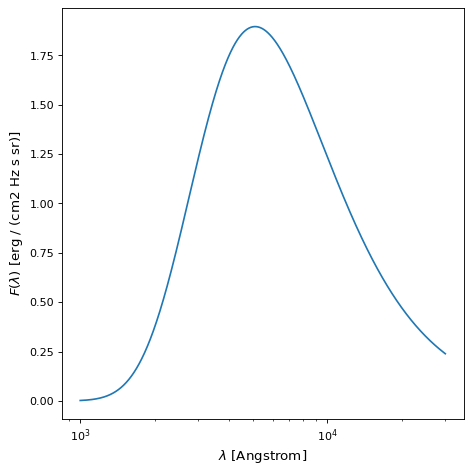
An example plot for a blackbody with a temperature of 10000 K and a scale of 1 is shown below. A scale of 1 shows the Planck function with no scaling in the default units returned by BlackBody.

import numpy as np
import matplotlib.pyplot as plt

from astropy.modeling.models import BlackBody
import astropy.units as u

wavelengths = np.logspace(np.log10(1000), np.log10(3e4), num=1000) * u.AA

# blackbody parameters
temperature = 10000 * u.K

# BlackBody provides the results in ergs/(cm^2 Hz s sr) when scale has no units
bb = BlackBody(temperature=temperature, scale=10000.0)
bb_result = bb(wavelengths)

fig, ax = plt.subplots(ncols=1)
ax.plot(wavelengths, bb_result, '-')

ax.set_xscale('log')
ax.set_xlabel(r"$\lambda$ [{}]".format(wavelengths.unit))
ax.set_ylabel(r"$F(\lambda)$ [{}]".format(bb_result.unit))

plt.tight_layout()
plt.show()

(png, svg, pdf)

The bolometric_flux() member function gives the bolometric flux using \(\sigma T^4/\pi\) where \(\sigma\) is the Stefan-Boltzmann constant.

The lambda_max() and nu_max() member functions give the wavelength and frequency of the maximum for \(B_\lambda\) and \(B_\nu\), respectively, calculated using Wein’s Law.

Note

Prior to v4.0, the BlackBody1D and the functions blackbody_nu and blackbody_lambda were provided. BlackBody1D was a more limited blackbody model that was specific to integrated fluxes from sources. The capabilities of all three can be obtained with BlackBody. See Blackbody Module (deprecated capabilities) and astropy issue #9066 for details.

Drude1D

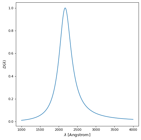
The Drude1D model provides a model for the behavior of an electron in a material (see Drude Model). Like the Lorentz1D model, the Drude model has broader wings than the Gaussian1D model. The Drude profile has been used to model dust features including the 2175 Angstrom extinction feature and the mid-infrared aromatic/PAH features. The Drude function at \(x\) is

\[D(x) = A \frac{(f/x_0)^2}{((x/x_0 - x_0/x)^2 + (f/x_0)^2}\]

where \(A\) is the amplitude, \(f\) is the full width at half maximum, and \(x_0\) is the central wavelength. An example of a Drude1D model with \(x_0 = 2175\) Angstrom and \(f = 400\) Angstrom is shown below.

import numpy as np
import matplotlib.pyplot as plt

from astropy.modeling.models import Drude1D
import astropy.units as u

wavelengths = np.linspace(1000, 4000, num=1000) * u.AA

# Parameters and model
mod = Drude1D(amplitude=1.0, x_0=2175. * u.AA, fwhm=400. * u.AA)
mod_result = mod(wavelengths)

fig, ax = plt.subplots(ncols=1)
ax.plot(wavelengths, mod_result, '-')

ax.set_xlabel(r"$\lambda$ [{}]".format(wavelengths.unit))
ax.set_ylabel(r"$D(\lambda)$")

plt.tight_layout()
plt.show()

(png, svg, pdf)