MODELS

Basics

The astropy.modeling package defines a number of models that are collected under a single namespace as astropy.modeling.models. Models behave like parametrized functions:

>>> import numpy as np
>>> from astropy.modeling import models
>>> g = models.Gaussian1D(amplitude=1.2, mean=0.9, stddev=0.5)
>>> print(g)
Model: Gaussian1D
Inputs: ('x',)
Outputs: ('y',)
Model set size: 1
Parameters:
    amplitude mean stddev
    --------- ---- ------
          1.2  0.9    0.5

Model parameters can be accessed as attributes:

>>> g.amplitude
Parameter('amplitude', value=1.2)
>>> g.mean
Parameter('mean', value=0.9)
>>> g.stddev  
Parameter('stddev', value=0.5, bounds=(1.1754943508222875e-38, None))

and can also be updated via those attributes:

>>> g.amplitude = 0.8
>>> g.amplitude
Parameter('amplitude', value=0.8)

Models can be evaluated by calling them as functions:

>>> g(0.1)
0.22242984036255528
>>> g(np.linspace(0.5, 1.5, 7))  
array([0.58091923, 0.71746405, 0.7929204 , 0.78415894, 0.69394278,
       0.54952605, 0.3894018 ])

As the above example demonstrates, in general most models evaluate array-like inputs according to the standard Numpy broadcasting rules for arrays. Models can therefore already be useful to evaluate common functions, independently of the fitting features of the package.

Instantiating and Evaluating Models

In general, models are instantiated by supplying the parameter values that define that instance of the model to the constructor, as demonstrated in the section on Parameters.

Additionally, a Model instance may represent a single model with one set of parameters, or a Model set consisting of a set of parameters each representing a different parameterization of the same parametric model. For example, you may instantiate a single Gaussian model with one mean, standard deviation, and amplitude. Or you may create a set of N Gaussians, each one of which would be evaluated on, for example, a different plane in an image cube.

For example, a single Gaussian model may be instantiated with all scalar parameters:

>>> from astropy.modeling.models import Gaussian1D
>>> g = Gaussian1D(amplitude=1, mean=0, stddev=1)
>>> g  
<Gaussian1D(amplitude=1., mean=0., stddev=1.)>

The newly created model instance g now works like a Gaussian function with the specific parameters. It takes a single input:

>>> g.inputs
('x',)
>>> g(x=0)
1.0

The model can also be called without explicitly using keyword arguments:

>>> g(0)
1.0

Or a set of Gaussians may be instantiated by passing multiple parameter values:

>>> from astropy.modeling.models import Gaussian1D
>>> gset = Gaussian1D(amplitude=[1, 1.5, 2],
...                   mean=[0, 1, 2],
...                   stddev=[1., 1., 1.],
...                   n_models=3)
>>> print(gset)  
Model: Gaussian1D
Inputs: ('x',)
Outputs: ('y',)
Model set size: 3
Parameters:
    amplitude mean stddev
    --------- ---- ------
          1.0  0.0    1.0
          1.5  1.0    1.0
          2.0  2.0    1.0

This model also works like a Gaussian function. The three models in the model set can be evaluated on the same input:

>>> gset(1.)
array([0.60653066, 1.5       , 1.21306132])

or on N=3 inputs:

>>> gset([1, 2, 3])
array([0.60653066, 0.90979599, 1.21306132])

For a comprehensive example of fitting a model set see Fitting Model Sets.

Model inverses

All models have a Model.inverse property which may, for some models, return a new model that is the analytic inverse of the model it is attached to. For example:

>>> from astropy.modeling.models import Linear1D
>>> linear = Linear1D(slope=0.8, intercept=1.0)
>>> linear.inverse
<Linear1D(slope=1.25, intercept=-1.25)>

The inverse of a model will always be a fully instantiated model in its own right, and so can be evaluated directly like:

>>> linear.inverse(2.0)
1.25

It is also possible to assign a custom inverse to a model. This may be useful, for example, in cases where a model does not have an analytic inverse, but may have an approximate inverse that was computed numerically and is represented by another model. This works even if the target model has a default analytic inverse–in this case the default is overridden with the custom inverse:

>>> from astropy.modeling.models import Polynomial1D
>>> linear.inverse = Polynomial1D(degree=1, c0=-1.25, c1=1.25)
>>> linear.inverse
<Polynomial1D(1, c0=-1.25, c1=1.25)>

If a custom inverse has been assigned to a model, it can be deleted with del model.inverse. This resets the inverse to its default (if one exists). If a default does not exist, accessing model.inverse raises a NotImplementedError. For example polynomial models do not have a default inverse:

>>> del linear.inverse
>>> linear.inverse
<Linear1D(slope=1.25, intercept=-1.25)>
>>> p = Polynomial1D(degree=2, c0=1.0, c1=2.0, c2=3.0)
>>> p.inverse
Traceback (most recent call last):
  File "<stdin>", line 1, in <module>
  File "astropy\modeling\core.py", line 796, in inverse
    raise NotImplementedError("An analytical inverse transform has not "
NotImplementedError: No analytical or user-supplied inverse transform
has been implemented for this model.

One may certainly compute an inverse and assign it to a polynomial model though.

Note

When assigning a custom inverse to a model no validation is performed to ensure that it is actually an inverse or even approximate inverse. So assign custom inverses at your own risk.

Bounding Boxes

Efficient Model Rendering with Bounding Boxes

All Model subclasses have a bounding_box attribute that can be used to set the limits over which the model is significant. This greatly improves the efficiency of evaluation when the input range is much larger than the characteristic width of the model itself. For example, to create a sky model image from a large survey catalog, each source should only be evaluated over the pixels to which it contributes a significant amount of flux. This task can otherwise be computationally prohibitive on an average CPU.

The Model.render method can be used to evaluate a model on an output array, or input coordinate arrays, limiting the evaluation to the bounding_box region if it is set. This function will also produce postage stamp images of the model if no other input array is passed. To instead extract postage stamps from the data array itself, see 2D Cutout Images.

Using the Bounding Box

For basic usage, see Model.bounding_box. By default no bounding_box is set, except on model subclasses where a bounding_box property or method is explicitly defined. The default is then the minimum rectangular region symmetric about the position that fully contains the model. If the model does not have a finite extent, the containment criteria are noted in the documentation. For example, see Gaussian2D.bounding_box.

Model.bounding_box can be set by the user to any callable. This is particularly useful for models created with custom_model or as a CompoundModel:

>>> from astropy.modeling import custom_model
>>> def ellipsoid(x, y, z, x0=0, y0=0, z0=0, a=2, b=3, c=4, amp=1):
...     rsq = ((x - x0) / a) ** 2 + ((y - y0) / b) ** 2 + ((z - z0) / c) ** 2
...     val = (rsq < 1) * amp
...     return val
...
>>> class Ellipsoid3D(custom_model(ellipsoid)):
...     # A 3D ellipsoid model
...     @property
...     def bounding_box(self):
...         return ((self.z0 - self.c, self.z0 + self.c),
...                 (self.y0 - self.b, self.y0 + self.b),
...                 (self.x0 - self.a, self.x0 + self.a))
...
>>> model = Ellipsoid3D()
>>> model.bounding_box
((-4.0, 4.0), (-3.0, 3.0), (-2.0, 2.0))

By default models are evaluated on any inputs. By passing a flag they can be evaluated only on inputs within the bounding box. For inputs outside of the bounding_box a fill_value is returned (np.nan by default):

>>> model(-5, 1, 1)
0.0
>>> model(-5, 1, 1, with_bounding_box=True)
nan
>>> model(-5, 1, 1, with_bounding_box=True, fill_value=-1)
-1.0

Warning

Currently when combining models the bounding boxes of components are combined only when joining models with the & operator. For the other operators bounding boxes for compound models must be assigned explicitly. A future release will determine the appropriate bounding box for a compound model where possible.

Efficient evaluation with Model.render()

When a model is evaluated over a range much larger than the model itself, it may be prudent to use the Model.render method if efficiency is a concern. The render method can be used to evaluate the model on an array of the same dimensions. model.render() can be called with no arguments to return a “postage stamp” of the bounding box region.

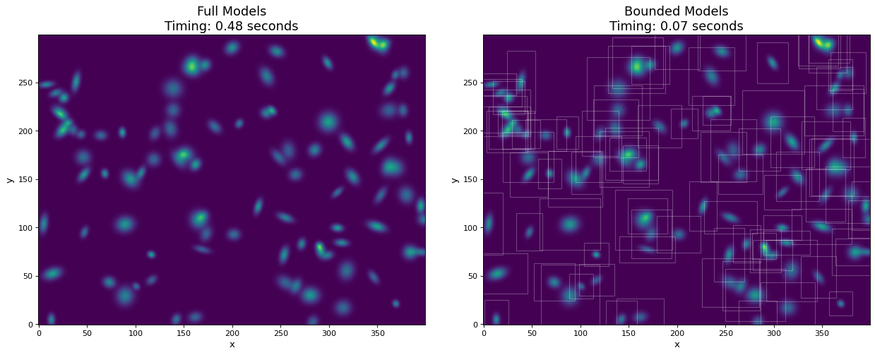
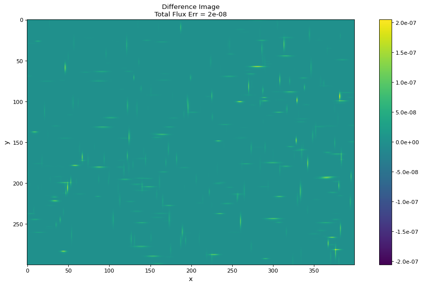
In this example, we generate a 300x400 pixel image of 100 2D Gaussian sources. For comparison, the models are evaluated both with and without using bounding boxes. By using bounding boxes, the evaluation speed increases by approximately a factor of 10 with negligible loss of information.

import numpy as np
from time import time
from astropy.modeling import models
import matplotlib.pyplot as plt
from matplotlib.patches import Rectangle

imshape = (300, 400)
y, x = np.indices(imshape)

# Generate random source model list
np.random.seed(0)
nsrc = 100
model_params = [
    dict(amplitude=np.random.uniform(.5, 1),
         x_mean=np.random.uniform(0, imshape[1] - 1),
         y_mean=np.random.uniform(0, imshape[0] - 1),
         x_stddev=np.random.uniform(2, 6),
         y_stddev=np.random.uniform(2, 6),
         theta=np.random.uniform(0, 2 * np.pi))
    for _ in range(nsrc)]

model_list = [models.Gaussian2D(**kwargs) for kwargs in model_params]

# Render models to image using bounding boxes
bb_image = np.zeros(imshape)
t_bb = time()
for model in model_list:
    model.render(bb_image)
t_bb = time() - t_bb

# Render models to image using full evaluation
full_image = np.zeros(imshape)
t_full = time()
for model in model_list:
    model.bounding_box = None
    model.render(full_image)
t_full = time() - t_full

flux = full_image.sum()
diff = (full_image - bb_image)
max_err = diff.max()

# Plots
plt.figure(figsize=(16, 7))
plt.subplots_adjust(left=.05, right=.97, bottom=.03, top=.97, wspace=0.15)

# Full model image
plt.subplot(121)
plt.imshow(full_image, origin='lower')
plt.title('Full Models\nTiming: {:.2f} seconds'.format(t_full), fontsize=16)
plt.xlabel('x')
plt.ylabel('y')

# Bounded model image with boxes overplotted
ax = plt.subplot(122)
plt.imshow(bb_image, origin='lower')
for model in model_list:
    del model.bounding_box  # Reset bounding_box to its default
    dy, dx = np.diff(model.bounding_box).flatten()
    pos = (model.x_mean.value - dx / 2, model.y_mean.value - dy / 2)
    r = Rectangle(pos, dx, dy, edgecolor='w', facecolor='none', alpha=.25)
    ax.add_patch(r)
plt.title('Bounded Models\nTiming: {:.2f} seconds'.format(t_bb), fontsize=16)
plt.xlabel('x')
plt.ylabel('y')

# Difference image
plt.figure(figsize=(16, 8))
plt.subplot(111)
plt.imshow(diff, vmin=-max_err, vmax=max_err)
plt.colorbar(format='%.1e')
plt.title('Difference Image\nTotal Flux Err = {:.0e}'.format(
    ((flux - np.sum(bb_image)) / flux)))
plt.xlabel('x')
plt.ylabel('y')
plt.show()

(png, svg, pdf)

(png, svg, pdf)

Model Separability

Simple models have a boolean Model.separable property. It indicates whether the outputs are independent and is essential for computing the separability of compound models using the is_separable() function. Having a separable compound model means that it can be decomposed into independent models, which in turn is useful in many applications. For example, it may be easier to define inverses using the independent parts of a model than the entire model. In other cases, tools using Generalized World Coordinate System (GWCS), can be more flexible and take advantage of separable spectral and spatial transforms.

Model Sets

In some cases it is useful to describe many models of the same type but with different sets of parameter values. This could be done simply by instantiating as many instances of a Model as are needed. But that can be inefficient for a large number of models. To that end, all model classes in astropy.modeling can also be used to represent a model set which is a collection of models of the same type, but with different values for their parameters.

To instantiate a model set, use argument n_models=N where N is the number of models in the set when constructing the model. The value of each parameter must be a list or array of length N, such that each item in the array corresponds to one model in the set:

>>> from astropy.modeling import models
>>> g = models.Gaussian1D(amplitude=[1, 2], mean=[0, 0],
...                       stddev=[0.1, 0.2], n_models=2)
>>> print(g)
Model: Gaussian1D
Inputs: ('x',)
Outputs: ('y',)
Model set size: 2
Parameters:
    amplitude mean stddev
    --------- ---- ------
          1.0  0.0    0.1
          2.0  0.0    0.2

This is equivalent to two Gaussians with the parameters amplitude=1, mean=0, stddev=0.1 and amplitude=2, mean=0, stddev=0.2 respectively. When printing the model the parameter values are displayed as a table, with each row corresponding to a single model in the set.

The number of models in a model set can be determined using the len builtin:

>>> len(g)
2

Single models have a length of 1, and are not considered a model set as such.

When evaluating a model set, by default the input must be the same length as the number of models, with one input per model:

>>> g([0, 0.1])  
array([1.        , 1.76499381])

The result is an array with one result per model in the set. It is also possible to broadcast a single input value to all models in the set:

>>> g(0)  
array([1., 2.])

Or when the input is an array:

>>> x = np.array([[0, 0, 0], [0.1, 0.1, 0.1]])
>>> print(x)
[[0.  0.  0. ]
 [0.1 0.1 0.1]]
>>> g(x)
array([[1.        , 1.        , 1.        ],
       [1.76499381, 1.76499381, 1.76499381]])

Internally the shape of the inputs, outputs, and parameter values is controlled by an attribute - model_set_axis. In the above case model_set_axis=0:

>>> g.model_set_axis
0

This indicates that elements along the 0-th axis will be passed as inputs to inidvidual models. Sometimes it may be useful to pass inputs along a different axis, for example the 1st axis:

>>> x = np.array([[0, 0, 0], [0.1, 0.1, 0.1]]).T
>>> print(x)
[[0.  0.1]
 [0.  0.1]
 [0.  0.1]]

Because there are two models in this model set and we are passing three inputs along the 0th axis, evaluation will fail:

>>> g(x)
Traceback (most recent call last):
...
ValueError: Input argument 'x' does not have the correct dimensions in
model_set_axis=0 for a model set with n_models=2.

There are two ways to get around this. model_set_axis can be passed in when the model is evaluated:

>>> g(x, model_set_axis=1)
array([[1.        , 1.76499381],
       [1.        , 1.76499381],
       [1.        , 1.76499381]])

Or when the model is initialized:

>>> g = models.Gaussian1D(amplitude=[[1, 2]], mean=[[0, 0]],
...                       stddev=[[0.1, 0.2]], n_models=2,
...                       model_set_axis=1)
>>> g(x)
array([[1.        , 1.76499381],
       [1.        , 1.76499381],
       [1.        , 1.76499381]])

Note that in the latter case, the shape of the individual parameters has changed to 2D because now the parameters are defined along the 1st axis.

The value of model_set_axis is either an integer number, representing the axis along which the different parameter sets and inputs are defined, or a boolean of value False, in which case it indicates all model sets should use the same inputs on evaluation. For example, the above model has a value of 1 for model_set_axis. If model_set_axis=False is passed the two models will be evaluated on the same input:

>>> g.model_set_axis
1
>>> result = g(x, model_set_axis=False)
>>> result
array([[[1.        , 0.60653066],
        [2.        , 1.76499381]],

       [[1.        , 0.60653066],
        [2.        , 1.76499381]],

       [[1.        , 0.60653066],
        [2.        , 1.76499381]]])
>>> result[: , 0]
array([[1.        , 0.60653066],
       [1.        , 0.60653066],
       [1.        , 0.60653066]])
>>> result[: , 1]
array([[2.        , 1.76499381],
       [2.        , 1.76499381],
       [2.        , 1.76499381]])

Currently model sets are most useful for fitting a set of linear models (example) allowing a large number of models of the same type to be fitted simultaneously (and independently from each other) to some large set of inputs, such as fitting a polynomial to the time response of each pixel in a data cube. This can greatly speed up the fitting process. The speed-up is due to solving the set of equations to find the exact solution. Nonlinear models, which require an iterative algorithm, cannot be currently fit using model sets. Model sets of nonlinear models can only be evaluated.

Model Serialization (Writing a Model to a File)

Models are serializable using the ASDF format. This can be useful in many contexts, one of which is the implementation of a Generalized World Coordinate System (GWCS).

Serializing a model to disk is possible by assigning the object to AsdfFile.tree:

>>> from asdf import AsdfFile
>>> from astropy.modeling import models
>>> rotation = models.Rotation2D(angle=23.7)
>>> f = AsdfFile()
>>> f.tree['model'] = rotation
>>> f.write_to('rotation.asdf')

To read the file and create the model:

>>> import asdf
>>> with asdf.open('rotation.asdf') as f:
...     model = f.tree['model']
>>> print(model)
Model: Rotation2D
Inputs: ('x', 'y')
Outputs: ('x', 'y')
Model set size: 1
Parameters:
    angle
    -----
     23.7

Compound models can also be serialized. Please note that some model attributes (e.g meta, tied parameter constraints used in fitting), as well as model sets are not yet serializable. For more information on serialization of models, see Details.