Fitting Models to Data

This module provides wrappers, called Fitters, around some Numpy and Scipy fitting functions. All Fitters can be called as functions. They take an instance of FittableModel as input and modify its parameters attribute. The idea is to make this extensible and allow users to easily add other fitters.

Linear fitting is done using Numpy’s numpy.linalg.lstsq function. There are currently two non-linear fitters which use scipy.optimize.leastsq and scipy.optimize.fmin_slsqp.

The rules for passing input to fitters are:

• Non-linear fitters currently work only with single models (not model sets).

• The linear fitter can fit a single input to multiple model sets creating multiple fitted models. This may require specifying the model_set_axis argument just as used when evaluating models; this may be required for the fitter to know how to broadcast the input data.

• The LinearLSQFitter currently works only with simple (not compound) models.

• The current fitters work only with models that have a single output (including bivariate functions such as Chebyshev2D but not compound models that map x, y -> x', y').

Simple 1-D model fitting

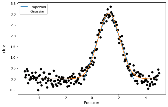
In this section, we look at a simple example of fitting a Gaussian to a simulated dataset. We use the Gaussian1D and Trapezoid1D models and the LevMarLSQFitter fitter to fit the data:

import numpy as np
import matplotlib.pyplot as plt
from astropy.modeling import models, fitting

# Generate fake data
np.random.seed(0)
x = np.linspace(-5., 5., 200)
y = 3 * np.exp(-0.5 * (x - 1.3)**2 / 0.8**2)
y += np.random.normal(0., 0.2, x.shape)

# Fit the data using a box model.
# Bounds are not really needed but included here to demonstrate usage.
t_init = models.Trapezoid1D(amplitude=1., x_0=0., width=1., slope=0.5,
                            bounds={"x_0": (-5., 5.)})
fit_t = fitting.LevMarLSQFitter()
t = fit_t(t_init, x, y)

# Fit the data using a Gaussian
g_init = models.Gaussian1D(amplitude=1., mean=0, stddev=1.)
fit_g = fitting.LevMarLSQFitter()
g = fit_g(g_init, x, y)

# Plot the data with the best-fit model
plt.figure(figsize=(8,5))
plt.plot(x, y, 'ko')
plt.plot(x, t(x), label='Trapezoid')
plt.plot(x, g(x), label='Gaussian')
plt.xlabel('Position')
plt.ylabel('Flux')
plt.legend(loc=2)

(png, svg, pdf)

As shown above, once instantiated, the fitter class can be used as a function that takes the initial model (t_init or g_init) and the data values (x and y), and returns a fitted model (t or g).

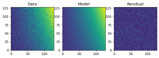
Simple 2-D model fitting

Similarly to the 1-D example, we can create a simulated 2-D data dataset, and fit a polynomial model to it. This could be used for example to fit the background in an image.

import warnings
import numpy as np
import matplotlib.pyplot as plt
from astropy.modeling import models, fitting

# Generate fake data
np.random.seed(0)
y, x = np.mgrid[:128, :128]
z = 2. * x ** 2 - 0.5 * x ** 2 + 1.5 * x * y - 1.
z += np.random.normal(0., 0.1, z.shape) * 50000.

# Fit the data using astropy.modeling
p_init = models.Polynomial2D(degree=2)
fit_p = fitting.LevMarLSQFitter()

with warnings.catch_warnings():
    # Ignore model linearity warning from the fitter
    warnings.simplefilter('ignore')
    p = fit_p(p_init, x, y, z)

# Plot the data with the best-fit model
plt.figure(figsize=(8, 2.5))
plt.subplot(1, 3, 1)
plt.imshow(z, origin='lower', interpolation='nearest', vmin=-1e4, vmax=5e4)
plt.title("Data")
plt.subplot(1, 3, 2)
plt.imshow(p(x, y), origin='lower', interpolation='nearest', vmin=-1e4,
           vmax=5e4)
plt.title("Model")
plt.subplot(1, 3, 3)
plt.imshow(z - p(x, y), origin='lower', interpolation='nearest', vmin=-1e4,
           vmax=5e4)
plt.title("Residual")

(png, svg, pdf)