SmoothlyBrokenPowerLaw1D

class astropy.modeling.powerlaws.SmoothlyBrokenPowerLaw1D(amplitude=1, x_break=1, alpha_1=- 2, alpha_2=2, delta=1, **kwargs)

Bases: astropy.modeling.Fittable1DModel

One dimensional smoothly broken power law model.

Parameters

amplitudefloat

Model amplitude at the break point.

x_breakfloat

Break point.

alpha_1float

Power law index for x << x_break.

alpha_2float

Power law index for x >> x_break.

deltafloat

Smoothness parameter.

See also

BrokenPowerLaw1D

Notes

Model formula (with \(A\) for amplitude, \(x_b\) for x_break, \(\alpha_1\) for alpha_1, \(\alpha_2\) for alpha_2 and \(\Delta\) for delta):

\[f(x) = A \left( \frac{x}{x_b} \right) ^ {-\alpha_1} \left\{ \frac{1}{2} \left[ 1 + \left( \frac{x}{x_b}\right)^{1 / \Delta} \right] \right\}^{(\alpha_1 - \alpha_2) \Delta}\]

The change of slope occurs between the values \(x_1\) and \(x_2\) such that:

\[\log_{10} \frac{x_2}{x_b} = \log_{10} \frac{x_b}{x_1} \sim \Delta\]

At values \(x \lesssim x_1\) and \(x \gtrsim x_2\) the model is approximately a simple power law with index \(\alpha_1\) and \(\alpha_2\) respectively. The two power laws are smoothly joined at values \(x_1 < x < x_2\), hence the \(\Delta\) parameter sets the “smoothness” of the slope change.

The delta parameter is bounded to values greater than 1e-3 (corresponding to \(x_2 / x_1 \gtrsim 1.002\)) to avoid overflow errors.

The amplitude parameter is bounded to positive values since this model is typically used to represent positive quantities.

Examples

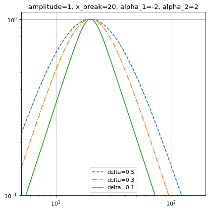
import numpy as np
import matplotlib.pyplot as plt
from astropy.modeling import models

x = np.logspace(0.7, 2.3, 500)
f = models.SmoothlyBrokenPowerLaw1D(amplitude=1, x_break=20,
                                    alpha_1=-2, alpha_2=2)

plt.figure()
plt.title("amplitude=1, x_break=20, alpha_1=-2, alpha_2=2")

f.delta = 0.5
plt.loglog(x, f(x), '--', label='delta=0.5')

f.delta = 0.3
plt.loglog(x, f(x), '-.', label='delta=0.3')

f.delta = 0.1
plt.loglog(x, f(x), label='delta=0.1')

plt.axis([x.min(), x.max(), 0.1, 1.1])
plt.legend(loc='lower center')
plt.grid(True)
plt.show()

(png, svg, pdf)

Attributes Summary

alpha_1
alpha_2
amplitude
delta
input_units	This property is used to indicate what units or sets of units the evaluate method expects, and returns a dictionary mapping inputs to units (or None if any units are accepted).
param_names
x_break

Methods Summary

evaluate(x, amplitude, x_break, alpha_1, …)	One dimensional smoothly broken power law model function
fit_deriv(x, amplitude, x_break, alpha_1, …)	One dimensional smoothly broken power law derivative with respect to parameters

Attributes Documentation

alpha_1 = Parameter('alpha_1', value=-2.0)

alpha_2 = Parameter('alpha_2', value=2.0)

amplitude = Parameter('amplitude', value=1.0, bounds=(0, None))

delta = Parameter('delta', value=1.0, bounds=(0.001, None))

input_units

This property is used to indicate what units or sets of units the evaluate method expects, and returns a dictionary mapping inputs to units (or None if any units are accepted).

Model sub-classes can also use function annotations in evaluate to indicate valid input units, in which case this property should not be overridden since it will return the input units based on the annotations.

param_names = ('amplitude', 'x_break', 'alpha_1', 'alpha_2', 'delta')

x_break = Parameter('x_break', value=1.0)

Methods Documentation

static evaluate(x, amplitude, x_break, alpha_1, alpha_2, delta)

One dimensional smoothly broken power law model function

static fit_deriv(x, amplitude, x_break, alpha_1, alpha_2, delta)

One dimensional smoothly broken power law derivative with respect to parameters